Defining subdomains for different materials
Solving PDEs in domains made up of different materials is a frequently encountered task. In FEniCS, these kinds of problems are handled by defining subdomains inside the domain. A simple example with two materials (subdomains) in 2D will demonstrate the idea. We consider the following variable-coefficient extension of the Poisson equation from the chapter Fundamentals: Solving the Poisson equation: $$ \begin{equation} \tag{4.4} -\nabla \cdot \left\lbrack \kappa(x,y)\nabla u(x,y)\right\rbrack = f(x, y), \end{equation} $$ in some domain \( \Omega \). Physically, this problem may be viewed as a model of heat conduction, with variable heat conductivity \( \kappa(x, y) \geq \underline{\kappa} > 0 \).
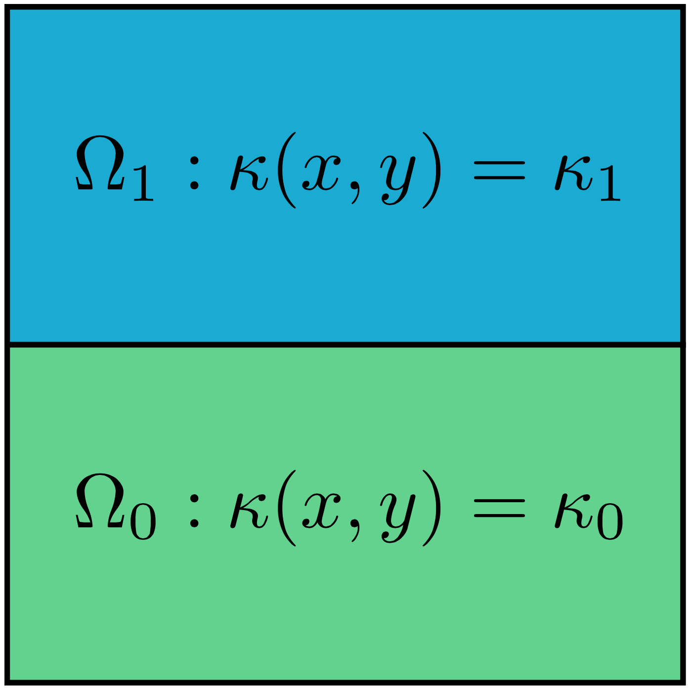
For illustration purposes, we consider the domain \( \Omega = [0,1]\times [0,1] \) and divide it into two equal subdomains, as depicted in Figure 12: $$ \begin{equation*} \Omega_0 = [0, 1]\times [0,1/2],\quad \Omega_1 = [0, 1]\times (1/2,1]\tp \end{equation*} $$ We define \( \kappa(x,y)=\kappa_0 \) in \( \Omega_0 \) and \( \kappa(x,y)=\kappa_1 \) in \( \Omega_1 \), where \( \kappa_0, \kappa_1 > 0 \) are given constants.
Figure 12: Two subdomains with different material parameters.
The variational formulation may be easily expressed in FEniCS as follows:
a = kappa*dot(grad(u), grad(v))*dx
L = f*v*dx
In the remainder of this section, we will discuss different strategies
for defining the coefficient kappa as an Expression that takes on
different values in the two subdomains.
Using expressions to define subdomains
The simplest way to implement a variable coefficient \( \kappa =
\kappa(x, y) \) is to define an Expression which depends on the
coordinates \( x \) and \( y \). We have previously used the Expression
class to define expressions based on simple formulas. Aternatively,
an Expression can be defined as a Python class which allows for more
complex logic. The following code snippet illustrates this
construction:
class K(Expression):
    def set_k_values(self, k_0, k_1):
        self.k_0, self.k_1 = k_0, k_1

    def eval(self, value, x):
        "Set value[0] to value at point x"
        tol = 1E-14
        if x[1] <= 0.5 + tol:
            value[0] = self.k_0
        else:
            value[0] = self.k_1

# Initialize kappa
kappa = K(degree=0)
kappa.set_k_values(1, 0.01)
The eval method gives great flexibility in defining functions, but a
downside is that FEniCS will call eval in Python for each node x,
which is a slow process.
An alternative method is to use a C++ string expression as we have seen before, which is much more efficient in FEniCS. This can be done using an inline if test:
tol = 1E-14
k_0 = 1.0
k_1 = 0.01
kappa = Expression('x[1] <= 0.5 + tol ? k_0 : k_1', degree=0,
               tol=tol, k_0=k_0, k_1=k_1)
This method of defining variable coefficients works if the subdomains are simple shapes that can be expressed in terms of geometric inequalities. However, for more complex subdomains, we will need to use a more general technique, as we will see next.
Using mesh functions to define subdomains
We now address how to specify the subdomains \( \Omega_0 \) and \( \Omega_1 \)
using a more general technique. This technique involves the use of two
classes that are essential in FEniCS when working with subdomains:
SubDomain and MeshFunction. Consider the following definition of the
boundary \( x = 0 \):
def boundary(x, on_boundary):
    tol = 1E-14
    return on_boundary and near(x[0], 0, tol)
This boundary definition is actually a shortcut to the more general
FEniCS concept SubDomain. A SubDomain is a class which defines a
region in space (a subdomain) in terms of a member function inside
which returns True for points that belong to the subdomain and
False for points that don't belong to the subdomain. Here is how to
specify the boundary \( x = 0 \) as a SubDomain:
class Boundary(SubDomain):
    def inside(self, x, on_boundary):
        tol = 1E-14
        return on_boundary and near(x[0], 0, tol)

boundary = Boundary()
bc = DirichletBC(V, Constant(0), boundary)
We notice that the inside function of the class Boundary is
(almost) identical to the previous boundary definition in terms of the
boundary function. Technically, our class Boundary is a
subclass of the FEniCS class SubDomain.
We will use two SubDomain subclasses to define the two subdomains
\( \Omega_0 \) and \( \Omega_1 \):
tol = 1E-14

class Omega_0(SubDomain):
    def inside(self, x, on_boundary):
        return x[1] <= 0.5 + tol

class Omega_1(SubDomain):
    def inside(self, x, on_boundary):
        return x[1] >= 0.5 - tol
Notice the use of <= and >= in both tests. FEniCS will call the
inside function for each vertex in a cell to determine whether or
not the cell belongs to a particular subdomain. For this reason, it is
important that the test holds for all vertices in cells aligned with
the boundary. In addition, we use a tolerance to make sure that
vertices on the internal boundary at \( y = 0.5 \) will belong to both
subdomains. This is a little counter-intuitive, but is necessary to
make the cells both above and below the internal boundary belong to
either \( \Omega_0 \) or \( \Omega_1 \).
To define the variable coefficient \( \kappa \), we will use a powerful tool in
FEniCS called a MeshFunction. A MeshFunction is a discrete
function that can be evaluated at a set of so-called mesh
entities. A mesh entity in FEniCS is either a vertex, an edge, a
face, or a cell (triangle or tetrahedron). A MeshFunction over cells
is suitable to represent subdomains (materials), while a
MeshFunction over facets (edges or faces) is used to represent
pieces of external or internal boundaries. A MeshFunction over cells
can also be used to represent boundary markers for mesh refinement. A
FEniCS MeshFunction is parameterized both over its data type (like
integers or booleans) and its dimension (0 = vertex, 1 = edge
etc.). Special subclasses VertexFunction, EdgeFunction etc. are
provided for easy definition of a MeshFunction of a particular
dimension.
Since we need to define subdomains of \( \Omega \) in the present example,
we make use of a CellFunction. The constructor
is given two arguments: (1) the type of value: 'int' for integers,
'size_t' for non-negative (unsigned) integers, 'double' for real
numbers, and 'bool' for logical values; (2) a Mesh object.
Alternatively, the constructor can take just a filename and initialize
the CellFunction from data in a file.
We first create a CellFunction with non-negative
integer values ('size_t'):
materials = CellFunction('size_t', mesh)
Next, we use the two subdomains to mark the cells belonging to each subdomain:
subdomain_0 = Omega_0()
subdomain_1 = Omega_1()
subdomain_0.mark(materials, 0)
subdomain_1.mark(materials, 1)
This will set the values of the mesh function materials to \( 0 \) on
each cell belonging to \( \Omega_0 \) and \( 1 \) on all cells belonging to
\( \Omega_1 \). Alternatively, we can use the following equivalent code to
mark the cells:
materials.set_all(0)
subdomain_1.mark(materials, 1)
To examine the values of the mesh function and see that we have indeed defined our subdomains correctly, we can simply plot the mesh function:
plot(materials, interactive=True)
We may also wish to store the values of the mesh function for later use:
File('materials.xml.gz') << materials
which can later be read back from file as follows:
File('materials.xml.gz') >> materials
Now, to use the values of the mesh function materials to define the
variable coefficient \( \kappa \), we create a FEniCS Expression:
class K(Expression):
    def __init__(self, materials, k_0, k_1, **kwargs):
        self.materials = materials
        self.k_0 = k_0
        self.k_1 = k_1

def eval_cell(self, values, x, cell):
        if self.materials[cell.index] == 0:
            values[0] = self.k_0
        else:
            values[0] = self.k_1

kappa = K(materials, k_0, k_1, degree=0)
This is similar to the Expression subclass we defined above, but we
make use of the member function eval_cell in place of the regular
eval function. This version of the evaluation function has an
additional cell argument which we can use to check on which cell we
are currently evaluating the function. We also defined the special
function __init__ (the constructor) so that we can pass all data to
the Expression when it is created.
Since we make use of geometric tests to define the two SubDomains
for \( \Omega_0 \) and \( \Omega_1 \), the MeshFunction method may seem like
an unnecessary complication of the simple method using an
Expression with an if-test. However, in general the definition of
subdomains may be available as a MeshFunction (from a data file),
perhaps generated as part of the mesh generation process, and not as a
simple geometric test. In such cases the method demonstrated here is
the recommended way to work with subdomains.
Using C++ code snippets to define subdomains
The SubDomain and Expression Python classes are very convenient,
but their use leads to function calls from C++ to Python for each node
in the mesh. Since this involves a significant cost, we need to make
use of C++ code if performance is an issue.
Instead of writing the SubDomain subclass in Python, we may instead use
the CompiledSubDomain tool in FEniCS to specify the subdomain in C++
code and thereby speed up our code. Consider
the definition of the classes Omega_0 and Omega_1 above in Python. The
key strings that define these subdomains can be expressed in C++ syntax
and given as arguments to CompiledSubDomain as follows:
tol = 1E-14
subdomain_0 = CompiledSubDomain('x[1] <= 0.5 + tol', tol=tol)
subdomain_1 = CompiledSubDomain('x[1] >= 0.5 - tol', tol=tol)
As seen, parameters can be specified using keyword arguments.
The resulting objects, subdomain_0 and subdomain_1, can be used
as ordinary SubDomain objects.
Compiled subdomain strings can be applied for specifying boundaries as well:
boundary_R = CompiledSubDomain('on_boundary && near(x[0], 1, tol)',
                               tol=1E-14)
It is also possible to feed the C++ string (without parameters)
directly as the third argument to DirichletBC without explicitly
constructing a CompiledSubDomain object:
bc1 = DirichletBC(V, value, 'on_boundary && near(x[0], 1, tol)')
Python Expression classes may also be redefined using C++ for more
efficient code. Consider again the definition of the class K above
for the variable coefficient \( \kappa = \kappa(x) \). This may be redefined using a
C++ code snippet and the keyword cppcode to the regular FEniCS
Expression class:
cppcode = """
class K : public Expression
{
public:

  void eval(Array<double>& values,
            const Array<double>& x,
            const ufc::cell& cell) const
  {
    if ((*materials)[cell.index] == 0)
      values[0] = k_0;
    else
      values[0] = k_1;
  }

  std::shared_ptr<MeshFunction<std::size_t>> materials;
  double k_0;
  double k_1;

};
"""

kappa = Expression(cppcode=cppcode, degree=0)
kappa.materials = materials
kappa.k_0 = k_0
kappa.k_1 = k_1